The algorithm

ERDR (article §1.1) works on a labelled sample E₀ = {S₁ … Sₘ} with heterogeneous features (quantitative set I, nominal set J) and classes K₁, K₂ (any number of classes works the same way: an enemy is an object of any other class). Each step below names the module that implements it and the workbook sheet that shows it.

Step 0 · scale unification and distances

Module erdr.core.distances · sheets Normalized Dataset, Zhuravlev Distances.

The article (§3): the quantitative features are normalized to [0; 1] before the Zhuravlev metric is applied. The default is the fractional-linear (min–max) transform over the objects of E₀ and the Zhuravlev metric:

x′ⱼ = (xⱼ − minⱼ) / (maxⱼ − minⱼ)         j ∈ I   (0 when maxⱼ = minⱼ)
ρ(S, S′) = Σ_{j∈I} |x′ⱼ − x′′ⱼ| + Σ_{j∈J} [xⱼ ≠ x′ⱼ]

Distances are rounded to 10 decimals (the quantitative part first, then the sum) so that equal distances tie exactly (ADR-008). Eight normalizers and twelve metrics can be chosen (Configuration).

Step 1 · four numbers for every object

Module erdr.core.characteristics · sheets Sorted Neighbors, ERDR Characteristics.

For Sᵢ ∈ K_t:

Symbol	Definition
r(Sᵢ)	min {ρ(Sᵢ, Sⱼ) : Sⱼ ∉ K_t} — the enemy radius
g(Sᵢ)	|{Sⱼ ∈ K_t : ρ(Sᵢ, Sⱼ) < r(Sᵢ)}| — own class strictly inside the sphere, Sᵢ included
z(Sᵢ, k)	the distance to the k-th nearest neighbour (Sᵢ excluded)
d(Sᵢ)	|z(Sᵢ, k) − r(Sᵢ)| / (z(Sᵢ, k) + r(Sᵢ)) — the priority (smaller = earlier)

Neighbours are sorted by (ρ, index): equal distances put the smaller index first. g counts Sᵢ itself, since ρ(Sᵢ, Sᵢ) = 0 < r(Sᵢ); the article confirms it — «g(Sⱼ) = 1 (т.е. Sⱼ остался единственным объектом в своей r(Sⱼ)-окрестности)». d is rounded to 10 decimals; d = 0 when z + r = 0 (ADR-008).

The k rule (ADR-005): odd k from k_min = 3 to k_max = 2·min|Kᵢ| − 3, from the class sizes of the sample — never hard-coded. Independently, z(Sᵢ, k) needs k ≤ m − 1 (k ≤ min|Kᵢ| − 1 for the own-class scope).

Step 2 · the priority queue

Sheet Priority Queue.

queue = {Sᵢ ∈ F | d(Sᵢ) ≥ 0}, ordered by d ↑, then r ↑, then index ↑

The order is static: the d and r of a waiting object never change; ERDR only takes objects out of the queue — from the front (the visited object is blocked) or from the middle (Step 5 moves an object to D before its turn). An empty queue ends the loop (Step 6).

Steps 3–5 · the main loop

Module erdr.core.algorithm · sheets ERDR Iterations, ERDR Trace.

1. Step 3 — take the first object Sᵢ of the queue.

2. Step 4 — build L, then block Sᵢ:

   L = {Sⱼ ∈ F ∩ K_t | ρ(Sⱼ, Sᵢ) < r(Sⱼ) and g(Sⱼ) > 1}
   d(Sᵢ) ← −(d(Sᵢ) + ε)                 (ε > 0; any ε gives the same result)
   |L| = 1  →  F ← F \ {Sᵢ},  D ← D ∪ {Sᵢ}
   

3. Step 5 — if |L| > 1, for every Sⱼ ∈ L (ascending index): g(Sⱼ) ← g(Sⱼ) − 1; if now g(Sⱼ) = 1, Sⱼ moves from F to D.

4. If |L| = 0 — not described in the article — Sᵢ is only blocked and stays in F.

Every iteration blocks one object, so ERDR stops after at most m iterations. Blocked objects stay in F: they can still be members of L and can still move to D later.

Steps 1–5 as hyperspheres

Module erdr.core.hyperspheres · sheets Hyperspheres (Step 1), Hyperspheres (Iterations), Hypersphere Data · all the figures.

Step 1 in geometric terms: every object Sᵢ is the centre of two spheres of the metric ρ.

Sphere	Radius	What it holds
enemy sphere (Sᵢ, r(Sᵢ)) — open	r(Sᵢ), through the nearest enemy	no enemy strictly inside; g(Sᵢ) counts the own class strictly inside, Sᵢ itself included
k-sphere (Sᵢ, z(Sᵢ, k)) — closed	z(Sᵢ, k), through the k-th neighbour	the k nearest neighbours (more on a tie)

Objects on the enemy sphere (ρ = r) are not counted, so a closed count ρ ≤ r differs from g by exactly them. d compares the two radii only:

q = min(r, z) / max(r, z)          d = |z − r| / (z + r) = (1 − q) / (1 + q)

d does not change when every distance is scaled; z = r ⇔ d = 0, and the Step 2 queue starts with the objects whose two spheres are closest in size. On the radius plane (r, z) d is constant on every line through the origin. With z over every class, the rank e of the nearest enemy decides: e = k ⇔ z = r, z < r gives g ≥ k + 1 and z > r gives g ≤ k − 1.

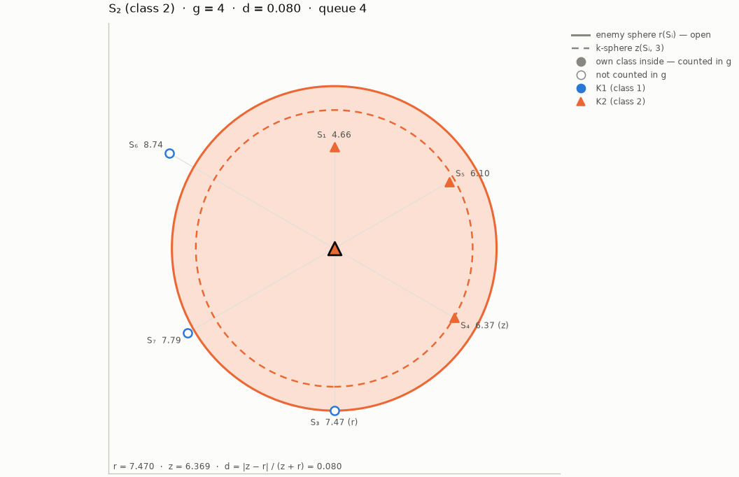
Steps 2–5 never change a sphere — only F and the counters g. The inverse view of the sphere matrix (its column of Sᵢ) lists the spheres that contain Sᵢ; when Sᵢ is selected, those of its own class still in F, with g > 1 and allowed by the readings A and B, form L:

Sⱼ ∈ L  ⇔  Sⱼ ∈ F ∩ K_t  and  r(Sⱼ) − ρ(Sⱼ, Sᵢ) > 0  and  g(Sⱼ) > 1  and  allowed by A, B

The iteration diagrams put Sᵢ in the centre and every object at its true distance ρ(Sⱼ, Sᵢ), so the sphere of Sⱼ contains the centre exactly when ρ(Sⱼ, Sᵢ) < r(Sⱼ): the spheres in L are solid and yellow, the others in F dashed, those of objects already in D dotted.

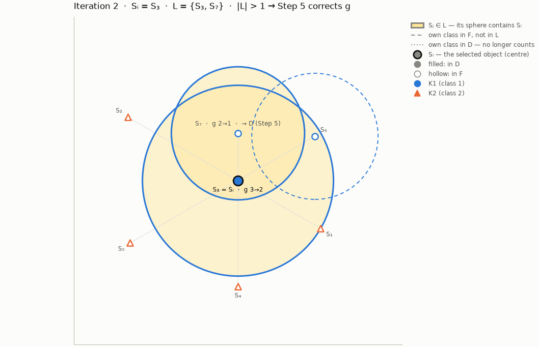
If an object coincides with an enemy, r = 0 and g = 0 (ADR-008): the object is not inside its own empty sphere, so in general g = [r > 0] + the own class strictly inside. The validator compares every value of the three sheets, and a property test checks on random samples with ties that the sphere test gives exactly the engine's L in every iteration (ADR-020).

Step 6 · the result

D = the training sample,   F = E₀ \ D = the validation sample

erdr.services.experiment.ExperimentResult.training_dataset and .validation_dataset are the two samples as datasets; run folders and the datasets export write them in the author's extended layout.

Readings: the open points

Module erdr.core.readings · sheets Readings (Switches), Article Table 1 Check.

Switch	Literal (1, default)	Alternative (2)	Configuration key
A — Sᵢ in its own L	yes, when g(Sᵢ) > 1 (ρ(Sᵢ, Sᵢ) = 0 < r(Sᵢ))	only Sⱼ ≠ Sᵢ	erdr.readings.self_in_l: included \| excluded
B — processed objects keep covering	yes, blocked objects stay in F	only Sᵢ and waiting objects can be in L	erdr.readings.blocked_cover: kept \| dropped
C — return to Step 2 in Step 5	after the whole L	right after the first move (L by ascending index)	erdr.readings.step5_return: after-all \| first-move
z — class scope of z(Sᵢ, k)	any class	own class only	erdr.readings.z_scope: all \| own-class

On the 7 default objects the eight readings of A, B, C give six different training samples (erdr readings). On all 270 objects (erdr sweep heart-disease-270):

k	Article Table 1	literal	B = 2	own-class z	B = 2 + own-class z	A = 2
3	75	198	81	194	75	124
5	77	190	73	192	76	121
7	77	201	72	202	71	130
13	104	177	84	179	88	106
17	102	165	90	173	94	100

No reading reproduces Table 1 exactly; the program behind it differs from the printed description in at least one detail (ADR-017).

The 17 cases

Module erdr.core.cases · sheet Case Checklist.

The workbook lists every situation the algorithm can be in — the k rule, border objects (g = 1), dense objects (g ≥ 2), both tie rules of Step 2, |L| = 1 with L = {Sᵢ} and with L = {Sⱼ}, |L| = 0, Step 5 with and without moves, moves of unprocessed and of processed objects, Sᵢ in its own L, a counter lowered twice, two moves in one Step 5, and the composition of D and F. detect_cases reports which occur in a run and where they first do; the default dataset shows all 17.

Notation

Objects, features and classes are shown 1-based — S₁, x₁, K1 — as in the article and the workbook; the code is 0-based (ADR-006). Sets print as {S₁, S₃}, the empty set as ∅, orders as S₁ → S₃.